BACK

GitHub repository
Kaggle

Topic Modelling of Banking Transactions using Latent Dirichlet Allocation (LDA)

Objective of the project

This is a personal project to get insights related to my personal expenses. In this notebook I analyze bank statements from my everyday banking account and my two credit cards using Topic Modelling with the idea to classify transactions. I also take a look on how my transactions have been affected by COVID 19.

In this notebook I am practicing my skills in:

• Pandas for working with files and datasets
• Seaborn and Ploty to plot the different figures
• Scikit-Learn - I use Latent Dirichlet Allocation (LDA) for analysis of the transactions description field

Considerations

• Data is available from Nov 2018. I will use data between Dec. 1st, 2018 and Sep. 30, 2020
• Transactions are made in Canadian dollars (CAD)
• If you would like to do a similar analysis, your personal bank has the option to export your transactions to a CSV file.

Funfact

I spent 172.89 CAD in coffee since Dec. 1, 2018. I love coffee!

Graphical summary of results

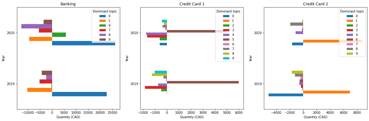
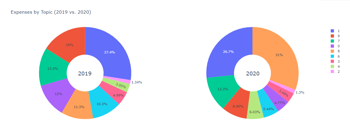
• The transactions from the 3 financial products were classified in 10 topics.

Contents

1. Pre-processing
2. Exploratory Data Analysis (EDA)
3. Topic Modelling
4. Visualization
5. Conclusions

Initial setup

• Import the needed packages: pandas, numpy and seaborn, matplotlib and plotly

import numpy as np
import pandas as pd
import seaborn as sns
import matplotlib.pyplot as plt

from plotly.subplots import make_subplots
import plotly.graph_objects as go
import plotly.offline as px

import datetime
import re   # Regular expressions

import nltk   # natural language tool kit
from sklearn.model_selection import GridSearchCV
from sklearn.feature_extraction.text import CountVectorizer
from sklearn.decomposition import LatentDirichletAllocation

import warnings
warnings.filterwarnings('ignore')

%matplotlib inline
print("Pandas version: ", pd.__version__)

# To export plotly figures in an HTML version of the jupyter notebook
px.init_notebook_mode()

Pandas version:  1.1.2

Pre-processing

• For the pre-processing of the data, the CSV files generated by the two different banks are read. Then, null values corresponding to "Transaction Type" are filled with value from "Transaction description". Finally, some features are added: year, month, day, week of year, weekday.

Read Dataset

# Read the dataset for Banking account
df_banking = pd.read_csv('banking.csv', header=None, usecols=[0, 1, 3, 4], names = ['Transaction Date', 'Quantity', 'Transaction description', 'Transaction Type'], parse_dates=['Transaction Date'])
df_banking = df_banking.set_index('Transaction Date')
print(f'Shape of dataframe: {df_banking.shape}')
df_banking = df_banking.sort_index()
df_banking.head()

Shape of dataframe: (704, 3)

	Quantity	Transaction description	Transaction Type
Transaction Date
2018-11-01	-550.00	WITHDRAWAL	MB-EMAIL MONEY TRF
2018-11-01	45.00	Miscellaneous Payment	PAYPAL
2018-11-01	-0.00	Service Charge	MB-FREE EMAIL MONEY TRF
2018-11-01	-50.00	Customer Transfer Dr.	MB-TRANSFER
2018-11-01	-37.91	Customer Transfer Dr.	MB-TRANSFER

# Read the dataset for credit card bank 1
df_creditcard_bank01 = pd.read_csv('bank01_creditcard.csv', header=None, names = ['Transaction Date', 'Transaction description', 'Quantity'],  parse_dates=['Transaction Date'])
df_creditcard_bank01 = df_creditcard_bank01.set_index('Transaction Date')
print(f'Shape of dataframe: {df_creditcard_bank01.shape}')
df_creditcard_bank01 = df_creditcard_bank01.sort_index()
df_creditcard_bank01.head()

Shape of dataframe: (559, 2)

	Transaction description	Quantity
Transaction Date
2018-11-02	ADOBE *PHOTOGPHY PLAN 8008336687 CA AMT ...	-15.18
2018-11-02	MB-CREDIT CARD/LOC PAY. FROM - 55376...	15.24
2018-11-03	MB-CREDIT CARD/LOC PAY. FROM - 55376...	57.80
2018-11-03	KOODO MOBILE PAC EDMONTON AB	-57.80
2018-11-04	AMZN Mktp CA*M84F08MK2 WWW.AMAZON.CAON	-38.98

# Read the dataset for credit card bank 2 and join them (In this case the transactions available are only last 25 months and you can download 12 months at a time)
df_creditcard_bank02a = pd.read_csv('bank02_creditcard_01.csv', usecols=[0, 3, 4, 5, 6], parse_dates=['Transaction Date'])
df_creditcard_bank02b = pd.read_csv('bank02_creditcard_02.csv', usecols=[0, 3, 4, 5, 6], parse_dates=['Transaction Date'])
df_creditcard_bank02 = pd.concat([df_creditcard_bank02a, df_creditcard_bank02b ])
df_creditcard_bank02 = df_creditcard_bank02.set_index('Transaction Date')

# Debit column should be negative
df_creditcard_bank02['Debit'] = -df_creditcard_bank02['Debit']
# Null values should be zero in Debit and credit columns. A new column 'Quantity' is created from Debit and Credit
df_creditcard_bank02.loc[df_creditcard_bank02['Debit'].isnull(), 'Debit'] = 0
df_creditcard_bank02.loc[df_creditcard_bank02['Credit'].isnull(), 'Credit'] = 0
df_creditcard_bank02['Quantity'] = df_creditcard_bank02['Debit'] + df_creditcard_bank02['Credit']

print(f'Shape of dataframe: {df_creditcard_bank02.shape}')
 
# df_creditcard_bank02 = df_creditcard_bank02.rename(columns={'Debit': 'Quantity'})
df_creditcard_bank02 = df_creditcard_bank02.sort_index()
df_creditcard_bank02.head()

Shape of dataframe: (370, 5)

	Description	Category	Debit	Credit	Quantity
Transaction Date
2018-10-27	COSTCO WHOLESALE W530	Merchandise	-317.69	0.00	-317.69
2018-10-30	PAYMENT	Payment/Credit	0.00	317.69	317.69
2018-10-31	PAYMENT	Payment/Credit	0.00	120.00	120.00
2018-11-15	INTEREST CHARGES	Fee/Interest Charge	-12.14	0.00	-12.14
2018-11-23	LACSA 1133M5A	Airfare	-1174.44	0.00	-1174.44

Check if there are null values

df_banking.info()

<class 'pandas.core.frame.DataFrame'>
DatetimeIndex: 704 entries, 2018-11-01 to 2020-10-13
Data columns (total 3 columns):
 #   Column                   Non-Null Count  Dtype  
---  ------                   --------------  -----  
 0   Quantity                 704 non-null    float64
 1   Transaction description  704 non-null    object 
 2   Transaction Type         678 non-null    object 
dtypes: float64(1), object(2)
memory usage: 22.0+ KB

# Fill NULL transaction type with "Transaction description"
df_banking['Transaction Type'] = df_banking['Transaction Type'].fillna(df_banking['Transaction description'])

df_creditcard_bank01.info()

<class 'pandas.core.frame.DataFrame'>
DatetimeIndex: 559 entries, 2018-11-02 to 2020-10-14
Data columns (total 2 columns):
 #   Column                   Non-Null Count  Dtype  
---  ------                   --------------  -----  
 0   Transaction description  559 non-null    object 
 1   Quantity                 559 non-null    float64
dtypes: float64(1), object(1)
memory usage: 13.1+ KB

df_creditcard_bank02.info()

<class 'pandas.core.frame.DataFrame'>
DatetimeIndex: 370 entries, 2018-10-27 to 2020-09-21
Data columns (total 5 columns):
 #   Column       Non-Null Count  Dtype  
---  ------       --------------  -----  
 0   Description  370 non-null    object 
 1   Category     370 non-null    object 
 2   Debit        370 non-null    float64
 3   Credit       370 non-null    float64
 4   Quantity     370 non-null    float64
dtypes: float64(3), object(2)
memory usage: 17.3+ KB

Addition of features for year, month , day

df_banking['Year'] = df_banking.index.year
df_banking['Month'] = df_banking.index.month
df_banking['Day'] = df_banking.index.day
df_banking['Week'] = df_banking.index.isocalendar().week  
df_banking['Weekday'] = df_banking.index.weekday

df_creditcard_bank01['Year'] = df_creditcard_bank01.index.year
df_creditcard_bank01['Month'] = df_creditcard_bank01.index.month
df_creditcard_bank01['Day'] = df_creditcard_bank01.index.day
df_creditcard_bank01['Week'] = df_creditcard_bank01.index.isocalendar().week  
df_creditcard_bank01['Weekday'] = df_creditcard_bank01.index.weekday

df_creditcard_bank02['Year'] = df_creditcard_bank02.index.year
df_creditcard_bank02['Month'] = df_creditcard_bank02.index.month
df_creditcard_bank02['Day'] = df_creditcard_bank02.index.day
df_creditcard_bank02['Week'] = df_creditcard_bank02.index.isocalendar().week 
df_creditcard_bank02['Weekday'] = df_creditcard_bank02.index.weekday

Exploratory Data Analysis (EDA)

Getting to know the dataset is very important. As initial steps I looked for the maximum and minimum transactions of each financial product. Then I looked for the available dates and general distribution of the transactions. I also checked how the transaction are distributed in time, month and day of the week. Finally, I compared IN/OUT transactions in 2019 period with the 2020 period as Sep. 30.

Maximum and minimum transactions

min_Banking = df_banking["Quantity"].min()
min_Banking_date = df_banking["Quantity"].idxmin() 
max_Banking = df_banking["Quantity"].max()
max_Banking_date = df_banking["Quantity"].idxmax()

print(f"The minimum value transaction for banking account was: {min_Banking} CAD on {min_Banking_date.date()}")
print(f"The maximum value transaction for banking account was: {max_Banking} CAD on {max_Banking_date.date()}")

The minimum value transaction for banking account was: -2250.0 CAD on 2020-09-18
The maximum value transaction for banking account was: 4312.17 CAD on 2020-03-30

min_Credit_bank01 = df_creditcard_bank01["Quantity"].min()
min_Credit_bank01_date = df_creditcard_bank01["Quantity"].idxmin() 
max_Credit_bank01 = df_creditcard_bank01["Quantity"].max()
max_Credit_bank01_date = df_creditcard_bank01["Quantity"].idxmax()

print(f"The minimum value transaction for banking account was: {min_Credit_bank01} CAD on {min_Credit_bank01_date.date()}")
print(f"The maximum value transaction for banking account was: {max_Credit_bank01} CAD on {max_Credit_bank01_date.date()}")

The minimum value transaction for banking account was: -327.68 CAD on 2020-06-01
The maximum value transaction for banking account was: 500.0 CAD on 2020-10-05

min_Credit_bank02 = df_creditcard_bank02["Quantity"].min()
min_Credit_bank02_date = df_creditcard_bank02["Quantity"].idxmin() 
max_Credit_bank02 = df_creditcard_bank02["Quantity"].max()
max_Credit_bank02_date = df_creditcard_bank02["Quantity"].idxmax()

print(f"The minimum value transaction for banking account was: {min_Credit_bank02} CAD on {min_Credit_bank02_date.date()}")
print(f"The maximum value transaction for banking account was: {max_Credit_bank02} CAD on {max_Credit_bank02_date.date()}")

The minimum value transaction for banking account was: -2189.1 CAD on 2019-11-29
The maximum value transaction for banking account was: 1220.0 CAD on 2020-03-04

Minimum date available

print(f"First available date of banking data is {df_banking.index[0].date()}")
print(f"First available date of credit card bank 1 data is {df_creditcard_bank01.index[0].date()}")
print(f"First available date of credit card bank 2 data is {df_creditcard_bank02.index[0].date()}")

First available date of banking data is 2018-11-01
First available date of credit card bank 1 data is 2018-11-02
First available date of credit card bank 2 data is 2018-10-27

Distribution plots

fig = make_subplots(rows=1, cols=3, subplot_titles=("Banking", "Credit Card 1", "Credit Card 2"))

fig.add_trace(
    go.Histogram(x=df_banking["Quantity"].values, name="Banking"), 
    row=1, col=1
)

fig.add_trace(
    go.Histogram(x=df_creditcard_bank01["Quantity"].values, name="Credit Card 1"),
    row=1, col=2
)

fig.add_trace(
    go.Histogram(x=df_creditcard_bank02["Quantity"].values, name="Credit Card 2"),
    row=1, col=3
)

fig.update_layout(height=400, width=800, title_text="Histograms for different financial products")
fig.update_xaxes(title_text="Quantity", row=1, col=1)
fig.update_xaxes(title_text="Quantity", row=1, col=2)
fig.update_xaxes(title_text="Quantity", row=1, col=3)
fig.update_yaxes(title_text="Count", row=1, col=1)

fig.update_traces(marker_line_width=1.5, opacity=0.6)

fig.show()

Transactions in time

# Create figure and plot space
fig, axes = plt.subplots(3, 1, figsize=(12, 15))
fig.subplots_adjust(hspace=0.5)

# For banking
axes[0].bar(df_banking.index.values, df_banking['Quantity'])
axes[1].bar(df_creditcard_bank01.index.values, df_creditcard_bank01['Quantity'])
axes[2].bar(df_creditcard_bank02.index.values, df_creditcard_bank02['Quantity']) 

# Set title and labels for axes
axes[0].set(xlabel="Date", ylabel="Quantity (CAD)", title="Banking transactions")
axes[1].set(xlabel="Date", ylabel="Quantity (CAD)", title="Credit card transactions from bank 1")
axes[2].set(xlabel="Date", ylabel="Quantity (CAD)", title="Credit card transactions from bank 2")

[Text(0.5, 0, 'Date'),
 Text(0, 0.5, 'Quantity (CAD)'),
 Text(0.5, 1.0, 'Credit card transactions from bank 2')]

Transactions by week and weekday

I am interested to see if the month, the day of the week, the day of month or the week of the year will make a difference

fig = make_subplots(rows=3, cols=1, subplot_titles=("Banking", "Credit Card 1", "Credit Card 2"))

fig.add_trace(
    go.Histogram(x=df_banking["Month"].values, name="Banking"), 
    row=1, col=1
)

fig.add_trace(
    go.Histogram(x=df_creditcard_bank01["Month"].values, name="Credit Card 1"),
    row=2, col=1
)

fig.add_trace(
    go.Histogram(x=df_creditcard_bank02["Month"].values, name="Credit Card 2"),
    row=3, col=1
)

fig.update_layout(height=800, width=800, title_text="Plot for different financial products in time")
fig.update_xaxes(title_text="Month", row=3, col=1)
fig.update_yaxes(title_text="Count", row=1, col=1)
fig.update_yaxes(title_text="Count", row=2, col=1)
fig.update_yaxes(title_text="Count", row=3, col=1)

fig.update_traces(marker_line_width=1.5, opacity=0.6)

fig.show()

fig = make_subplots(rows=3, cols=1, subplot_titles=("Banking", "Credit Card 1", "Credit Card 2"))

fig.add_trace(
    go.Histogram(x=df_banking["Day"].values, name="Banking"), 
    row=1, col=1
)

fig.add_trace(
    go.Histogram(x=df_creditcard_bank01["Day"].values, name="Credit Card 1"),
    row=2, col=1
)

fig.add_trace(
    go.Histogram(x=df_creditcard_bank02["Day"].values, name="Credit Card 2"),
    row=3, col=1
)

fig.update_layout(height=800, width=800, title_text="Plot for different financial products in time")
fig.update_xaxes(title_text="Day", row=3, col=1)
fig.update_yaxes(title_text="Count", row=1, col=1)
fig.update_yaxes(title_text="Count", row=2, col=1)
fig.update_yaxes(title_text="Count", row=3, col=1)

fig.update_traces(marker_line_width=1.5, opacity=0.6)
fig.show()

fig = make_subplots(rows=3, cols=1, subplot_titles=("Banking", "Credit Card 1", "Credit Card 2"))

fig.add_trace(
    go.Histogram(x=df_banking["Week"].values, name="Banking"), 
    row=1, col=1
)

fig.add_trace(
    go.Histogram(x=df_creditcard_bank01["Week"].values, name="Credit Card 1"),
    row=2, col=1
)

fig.add_trace(
    go.Histogram(x=df_creditcard_bank02["Week"].values, name="Credit Card 2"),
    row=3, col=1
)

fig.update_layout(height=800, width=800, title_text="Plot for different financial products in time")
fig.update_xaxes(title_text="Week", row=3, col=1)
fig.update_yaxes(title_text="Count", row=1, col=1)
fig.update_yaxes(title_text="Count", row=2, col=1)
fig.update_yaxes(title_text="Count", row=3, col=1)

fig.update_traces(marker_line_width=1.5, opacity=0.6)
fig.show()

fig = make_subplots(rows=3, cols=1, subplot_titles=("Banking", "Credit Card 1", "Credit Card 2"))

fig.add_trace(
    go.Histogram(x=df_banking["Weekday"].values, name="Banking"), 
    row=1, col=1
)

fig.add_trace(
    go.Histogram(x=df_creditcard_bank01["Weekday"].values, name="Credit Card 1"),
    row=2, col=1
)

fig.add_trace(
    go.Histogram(x=df_creditcard_bank02["Weekday"].values, name="Credit Card 2"),
    row=3, col=1
)

fig.update_layout(height=800, width=800, title_text="Plot for different financial products in time")
fig.update_xaxes(title_text="Weekday", row=3, col=1)
fig.update_yaxes(title_text="Count", row=1, col=1)
fig.update_yaxes(title_text="Count", row=2, col=1)
fig.update_yaxes(title_text="Count", row=3, col=1)

fig.update_traces(marker_line_width=1.5, opacity=0.6)
fig.show()

Comparision 2019 vs 2020

df_banking.head()

	Quantity	Transaction description	Transaction Type	Year	Month	Day	Week	Weekday
Transaction Date
2018-11-01	-550.00	WITHDRAWAL	MB-EMAIL MONEY TRF	2018	11	1	44	3
2018-11-01	45.00	Miscellaneous Payment	PAYPAL	2018	11	1	44	3
2018-11-01	-0.00	Service Charge	MB-FREE EMAIL MONEY TRF	2018	11	1	44	3
2018-11-01	-50.00	Customer Transfer Dr.	MB-TRANSFER	2018	11	1	44	3
2018-11-01	-37.91	Customer Transfer Dr.	MB-TRANSFER	2018	11	1	44	3

# Transactions in 2019
df_2019_credit02_IN = df_creditcard_bank01[ (df_creditcard_bank01['Year'] == 2019) & (df_creditcard_bank01['Quantity'] > 0 )]
df_2019_credit02_OUT = df_creditcard_bank01[ (df_creditcard_bank01['Year'] == 2019) & (df_creditcard_bank01['Quantity'] < 0 )]

df_2019_credit02_IN

	Transaction description	Quantity	Year	Month	Day	Week	Weekday
Transaction Date
2019-01-02	MB-CREDIT CARD/LOC PAY. FROM - 55376...	15.82	2019	1	2	1	2
2019-01-03	MB-CREDIT CARD/LOC PAY. FROM - 55376...	438.75	2019	1	3	1	3
2019-01-03	MB-CREDIT CARD/LOC PAY. FROM - 55376...	35.00	2019	1	3	1	3
2019-01-05	MB-CREDIT CARD/LOC PAY. FROM - 55376...	57.80	2019	1	5	1	5
2019-01-11	MB-CREDIT CARD/LOC PAY. FROM - 55376...	60.12	2019	1	11	2	4
...	...	...	...	...	...	...	...
2019-11-29	MB-CREDIT CARD/LOC PAY. FROM - 55376...	20.58	2019	11	29	48	4
2019-12-07	MB-CREDIT CARD/LOC PAY. FROM - 55376...	193.39	2019	12	7	49	5
2019-12-10	MB-CREDIT CARD/LOC PAY. FROM - 55376...	12.46	2019	12	10	50	1
2019-12-20	MB-CREDIT CARD/LOC PAY. FROM - 55376...	105.02	2019	12	20	51	4
2019-12-31	MB-CREDIT CARD/LOC PAY. FROM - 55376...	85.00	2019	12	31	1	1

68 rows × 7 columns

data = [
    [2019, df_banking[ (df_banking['Year'] == 2019) & (df_banking['Quantity'] > 0 )]['Quantity'].sum(),  -df_banking[ (df_banking['Year'] == 2019) & (df_banking['Quantity'] < 0 )]['Quantity'].sum(), 'Banking'],
    [2019, df_creditcard_bank01[ (df_creditcard_bank01['Year'] == 2019) & (df_creditcard_bank01['Quantity'] > 0 )]['Quantity'].sum(),  -df_creditcard_bank01[ (df_creditcard_bank01['Year'] == 2019) & (df_creditcard_bank01['Quantity'] < 0 )]['Quantity'].sum(), 'Credit Card Bank 1'],
    [2019, df_creditcard_bank02[ (df_creditcard_bank02['Year'] == 2019) & (df_creditcard_bank02['Quantity'] > 0 )]['Quantity'].sum(),  -df_creditcard_bank02[ (df_creditcard_bank02['Year'] == 2019) & (df_creditcard_bank02['Quantity'] < 0 )]['Quantity'].sum(), 'Credit Card Bank 2'],
    [2020, df_banking[ (df_banking['Year'] == 2020) & (df_banking['Quantity'] > 0 )]['Quantity'].sum(),  -df_banking[ (df_banking['Year'] == 2020) & (df_banking['Quantity'] < 0 )]['Quantity'].sum(), 'Banking'],
    [2020, df_creditcard_bank01[ (df_creditcard_bank01['Year'] == 2020) & (df_creditcard_bank01['Quantity'] > 0 )]['Quantity'].sum(),  -df_creditcard_bank01[ (df_creditcard_bank01['Year'] == 2020) & (df_creditcard_bank01['Quantity'] < 0 )]['Quantity'].sum(), 'Credit Card Bank 1'],
    [2020, df_creditcard_bank02[ (df_creditcard_bank02['Year'] == 2020) & (df_creditcard_bank02['Quantity'] > 0 )]['Quantity'].sum(),  -df_creditcard_bank02[ (df_creditcard_bank02['Year'] == 2020) & (df_creditcard_bank02['Quantity'] < 0 )]['Quantity'].sum(), 'Credit Card Bank 2']    
 ]

df_transactionsSummary = pd.DataFrame(data = data, columns=['Year', 'IN', 'OUT', 'Origin'])
df_transactionsSummary['Difference'] = df_transactionsSummary['IN'] - df_transactionsSummary['OUT']
df_transactionsSummary

	Year	IN	OUT	Origin	Difference
0	2019	28018.69	27639.28	Banking	379.41
1	2019	6094.79	5796.53	Credit Card Bank 1	298.26
2	2019	6954.62	9950.12	Credit Card Bank 2	-2995.50
3	2020	39224.44	39765.53	Banking	-541.09
4	2020	6579.79	6556.54	Credit Card Bank 1	23.25
5	2020	8784.65	5146.45	Credit Card Bank 2	3638.20

change_bank = df_transactionsSummary[df_transactionsSummary['Origin'] == "Banking"]['IN'].reset_index(drop=True).values
change_CC1 = df_transactionsSummary[df_transactionsSummary['Origin'] == "Credit Card Bank 1"]['OUT'].reset_index(drop=True).values
change_CC2 = df_transactionsSummary[df_transactionsSummary['Origin'] == "Credit Card Bank 2"]['OUT'].reset_index(drop=True).values

print('Debt (IN):', "{:.2f}".format(100*(change_bank[1] - change_bank[0])/change_bank[0]) + '%' )
print('Credit Card 1 (OUT):', "{:.2f}".format(100*(change_CC1[1] - change_CC1[0])/change_CC1[0]) + '%')
print('Credit Card 2 (OUT):', "{:.2f}".format(100*(change_CC2[1] - change_CC2[0])/change_CC2[0]) + '%')

Debt (IN): 39.99%
Credit Card 1 (OUT): 13.11%
Credit Card 2 (OUT): -48.28%

df_transactionsSummary_banking = df_transactionsSummary[df_transactionsSummary['Origin'] == 'Banking']
import plotly.express as px
fig = px.bar(df_transactionsSummary_banking, x="Year", y=["IN", "OUT"],
             labels={                     
                     "value": "Quantity (CAD)",
                     "variable": "Type"
                 },
              barmode='group',
             height=400, width=600)

fig.update_traces(marker_line_width=1.5, opacity=0.6)
fig.update_layout(title_text='Quantity of Debit Transactions - 2019 vs 2020')

fig.show()

df_transactionsSummary_CC1 = df_transactionsSummary[df_transactionsSummary['Origin'] == 'Credit Card Bank 1']
import plotly.express as px
fig = px.bar(df_transactionsSummary_CC1, x="Year", y=["IN", "OUT"],
              labels={                     
                     "value": "Quantity (CAD)",
                     "variable": "Type"
                 },
              barmode='group',
             height=400, width=600)

fig.update_traces(marker_line_width=1.5, opacity=0.6)
fig.update_layout(title_text='Quantity of Credit Card Transactions (Bank 1) - 2019 vs 2020')

fig.show()

df_transactionsSummary_CC2 = df_transactionsSummary[df_transactionsSummary['Origin'] == 'Credit Card Bank 2']

fig = px.bar(df_transactionsSummary_CC2, x="Year", y=["IN", "OUT"],
              labels={                     
                     "value": "Quantity (CAD)",
                     "variable": "Type"
                 },
              barmode='group',
             height=400, width=600)

fig.update_traces(marker_line_width=1.5, opacity=0.6)
fig.update_layout(title_text='Quantity of Credit Card Transactions (Bank 2) - 2019 vs 2020')

fig.show()

Some conclusion from EDA

• The months where I made more transactions were January and December. A peak in June/July can also be observed. This is consistent with Summer and Christmas seasons

Comparing 2019 vs. 2020 (up to Sep. 30)

• Quantity of IN debit transactions in 2020 had increased in 39.99%
• Quantity of Output credit card transactions from bank 1 (limit 1000 CAD) had increased in 13.11%
• Quantity of Output credit card transactions from bank 2 (limit 5000 CAD) had decreased in 48.28%

Topic Modelling

The idea of Topic Modelling in Natural Language Processing is to discover abstract topics in documents. The Latent Dirichlet Allocation (LDA) is a generative statistical model that allows sets of observations to be explained by unobserved groups. This is within the Unsupervised Learning category. Some examples can be found here: Example 1, Example 2, Example 3

Some preparation is needed first.

Pre preposing

Selection of dates of interest

• Data is available from different dates according to the financial product. The selected dates are from Dec 1, 2018 to Sep 30, 2020

date01 = datetime.date(2018, 12, 1)
date02 = datetime.date(2020, 9, 30)
df_banking = df_banking[(df_banking.index.date >= date01) & (df_banking.index.date <= date02)]
df_creditcard_bank01 = df_creditcard_bank01[(df_creditcard_bank01.index.date >= date01) & (df_creditcard_bank01.index.date <= date02)]
df_creditcard_bank02 = df_creditcard_bank02[(df_creditcard_bank02.index.date >= date01) & (df_creditcard_bank02.index.date <= date02)]

Quick view on description fields

A quick look on the description field show us that we can use it to help the classification of transactions. It is interesting that Bank 2 provides a category field. For this study that column won't be used.

df_banking['Transaction description'].unique()[:5]

array(['Bill Payment           ', 'POS Purchase           ',
       'DEPOSIT                ', 'ABM Withdrawal',
       'Miscellaneous Payment  '], dtype=object)

df_banking['Transaction Type'].unique()[:5]

array(['MB-SCOTIA SCENE VISA CARD', 'FPOS TIM HORTONS #0604# QSTRAT',
       'FPOS THE BOOK STORE AT WELONDO', 'GPOS CENTRE SPOT         LONDO',
       'GPOS ENGINEERING         LONDO'], dtype=object)

df_creditcard_bank01['Transaction description'].unique()[:5]

array(['MB-CREDIT CARD/LOC PAY.           FROM - 553760500321 ',
       'LATINO MARKET HERMIDA INCLONDON       ON  (GOOGLE PAY) ',
       'SHOPPERS DRUG MART0765   LONDON       ON  (GOOGLE PAY) ',
       'DOLLARAMA # 336          LONDON       ON  (GOOGLE PAY) ',
       'UberBV                   Amsterdam    ON '], dtype=object)

df_creditcard_bank02['Description'].unique()[:5]

array(['PAYMENT', 'INTEREST CHARGE ADJUSTMENT', 'INTEREST CHARGES',
       'COSTCO WHOLESALE W530', 'EXITO SANTA MARTA CENT'], dtype=object)

# Category field for second credit card wont be used
categories_CC2 = df_creditcard_bank02['Category'].unique()
print(categories_CC2.shape)
categories_CC2

(14,)

array(['Payment/Credit', 'Fee/Interest Charge', 'Merchandise', 'Dining',
       'Lodging', 'Health Care', 'Gas/Automotive', 'Other',
       'Other Services', 'Entertainment', 'Other Travel', 'Phone/Cable',
       'Professional Services', 'Airfare'], dtype=object)

df_banking[['Transaction description', 'Transaction Type', 'Year', 'Quantity']].groupby(['Transaction description', 'Transaction Type', 'Year']).sum().head()

			Quantity
Transaction description	Transaction Type	Year
ABM Deposit	ABM Deposit	2019	1166.80
ABM Withdrawal	ABM Withdrawal	2018	-240.00
		2019	-686.45
		2020	-62.00
Accounts Payable	UNIVERSITY OF WESTERN ONTARIO	2019	961.57

df_creditcard_bank01[['Transaction description', 'Year', 'Quantity']].groupby(['Transaction description', 'Year']).sum().head()

		Quantity
Transaction description	Year
168 SUSHI ASIAN BUFFET LONDON ON	2019	-79.47
64053 MACS CONV. STORES MOUNT BRYDGESON	2020	-120.66
A&W #4614 LISTOWEL ON	2019	-27.75
ADOBE *PHOTOGPHY PLAN 8008336687 CA AMT 11.29 UNITED STATES DOLLAR	2018	-15.44
	2019	-154.69

df_creditcard_bank02[['Description', 'Year', 'Quantity']].groupby(['Description', 'Year']).sum().head()

		Quantity
Description	Year
#293 SPORT CHEK	2019	-6.53
01013 MACS CONV. STORE	2019	-5.40
168 SUSHI ASIAN BUFFET	2019	-84.47
64053 MAC'S CONVENIE	2019	-41.89
64053 MACS CONV. STORE	2019	-267.74

Joining the data

I will join the three data sets. A new column corresponding to the original dataset will be created

df_banking['Original DF'] = 'Banking'
df_creditcard_bank01['Original DF'] = 'Credit Card - Bank 1'
df_creditcard_bank02['Original DF'] = 'Credit Card - Bank 2'

df_transactions_01a = df_banking.copy()
df_transactions_01a = df_transactions_01a.drop(columns=['Transaction Type'])
df_transactions_01a = df_transactions_01a.reset_index()

df_transactions_01b = df_creditcard_bank01.copy()
df_transactions_01b = df_transactions_01b.reset_index()

df_transactions_01c = df_creditcard_bank02.copy()
df_transactions_01c = df_transactions_01c.drop(columns=['Category', 'Debit', 'Credit'])
df_transactions_01c = df_transactions_01c.rename(columns={'Description': 'Transaction description'})
df_transactions_01c = df_transactions_01c.reset_index()

df_transactions_01b

	Transaction Date	Transaction description	Quantity	Year	Month	Day	Week	Weekday	Original DF
0	2018-12-01	MB-CREDIT CARD/LOC PAY. FROM - 55376...	72.50	2018	12	1	48	5	Credit Card - Bank 1
1	2018-12-01	MB-CREDIT CARD/LOC PAY. FROM - 55376...	68.00	2018	12	1	48	5	Credit Card - Bank 1
2	2018-12-01	MB-CREDIT CARD/LOC PAY. FROM - 55376...	12.78	2018	12	1	48	5	Credit Card - Bank 1
3	2018-12-01	LATINO MARKET HERMIDA INCLONDON ON (GOO...	-72.50	2018	12	1	48	5	Credit Card - Bank 1
4	2018-12-01	SHOPPERS DRUG MART0765 LONDON ON (GOO...	-32.77	2018	12	1	48	5	Credit Card - Bank 1
...	...	...	...	...	...	...	...	...	...
504	2020-09-27	WINNERS 441 COLLINGWOOD ON	-42.91	2020	9	27	39	6	Credit Card - Bank 1
505	2020-09-27	STAPLES/BUSINESS DEPOT COLLINGWOOD ON	-37.02	2020	9	27	39	6	Credit Card - Bank 1
506	2020-09-28	DOLLARAMA #1222 KOMOKA ON	-30.31	2020	9	28	40	0	Credit Card - Bank 1
507	2020-09-28	JOLLEY`S DAIRY BAR &VIDEOFLESHERTON ON	-3.75	2020	9	28	40	0	Credit Card - Bank 1
508	2020-09-29	MB-CREDIT CARD/LOC PAY. FROM - 55376...	100.00	2020	9	29	40	1	Credit Card - Bank 1

509 rows × 9 columns

frames = [df_transactions_01a, df_transactions_01b, df_transactions_01c]
df_transactions = pd.concat(frames)
df_transactions = df_transactions.reset_index().drop(columns='index').sort_values(['Transaction Date']).reset_index().drop(columns='index')

df_transactions.head()

	Transaction Date	Quantity	Transaction description	Year	Month	Day	Week	Weekday	Original DF
0	2018-12-01	-68.00	Bill Payment	2018	12	1	48	5	Banking
1	2018-12-01	12.78	MB-CREDIT CARD/LOC PAY. FROM - 55376...	2018	12	1	48	5	Credit Card - Bank 1
2	2018-12-01	-72.50	LATINO MARKET HERMIDA INCLONDON ON (GOO...	2018	12	1	48	5	Credit Card - Bank 1
3	2018-12-01	-32.77	SHOPPERS DRUG MART0765 LONDON ON (GOO...	2018	12	1	48	5	Credit Card - Bank 1
4	2018-12-01	-22.94	DOLLARAMA # 336 LONDON ON (GOO...	2018	12	1	48	5	Credit Card - Bank 1

Text Analysis for Transaction description field

Pre-processing

Within the transaction description, we can see items with numbers, for example for transactions related with Dollarama have associated a number corresponding to the store. However, for this analysis what I want to know is the category of the expense and not the place. In that sense, the 'Transaction description' is converted to lower case and the numbers and symbols are eliminated.

It is important to 'clean' the transaction description field as follows:

• Making the transaction description lower case
• Erasing the special characters
• Remove stop words

df_transactions[df_transactions['Transaction description'].str.contains('DOLLARAMA')].head()

	Transaction Date	Quantity	Transaction description	Year	Month	Day	Week	Weekday	Original DF
4	2018-12-01	-22.94	DOLLARAMA # 336 LONDON ON (GOO...	2018	12	1	48	5	Credit Card - Bank 1
113	2019-01-17	-15.59	DOLLARAMA # 485 LONDON ON (GOO...	2019	1	17	3	3	Credit Card - Bank 1
164	2019-02-17	-9.66	DOLLARAMA # 291 STRATHROY ON	2019	2	17	7	6	Credit Card - Bank 1
204	2019-03-16	-24.01	DOLLARAMA #1222 KOMOKA ON	2019	3	16	11	5	Credit Card - Bank 1
258	2019-04-06	-14.69	DOLLARAMA #1075 LONDON ON	2019	4	6	14	5	Credit Card - Bank 1

# lowercase
df_transactions['Transaction description'] = df_transactions['Transaction description'].str.lower()

# Erasing special characters
df_transactions['Transaction description'] = df_transactions['Transaction description'].str.replace('*', ' ')
df_transactions['Transaction description'] = df_transactions['Transaction description'].str.replace('.', ' ')
df_transactions['Transaction description'] = df_transactions['Transaction description'].apply(lambda x: re.sub(r'[^a-zA-Z\s\']+', ' ', x))

df_transactions[df_transactions['Transaction description'].str.contains('dollarama')].head()

	Transaction Date	Quantity	Transaction description	Year	Month	Day	Week	Weekday	Original DF
4	2018-12-01	-22.94	dollarama london on googl...	2018	12	1	48	5	Credit Card - Bank 1
113	2019-01-17	-15.59	dollarama london on googl...	2019	1	17	3	3	Credit Card - Bank 1
164	2019-02-17	-9.66	dollarama strathroy on	2019	2	17	7	6	Credit Card - Bank 1
204	2019-03-16	-24.01	dollarama komoka on	2019	3	16	11	5	Credit Card - Bank 1
258	2019-04-06	-14.69	dollarama london on	2019	4	6	14	5	Credit Card - Bank 1

# Removing stop words
nltk.download('stopwords')
from nltk.corpus import stopwords
stop_words = set(stopwords.words('english'))

df_transactions['Transaction description'] = df_transactions['Transaction description'].apply(lambda x: [word for word in x.split() if word not in stop_words])
df_transactions['Transaction description'] = [' '.join(map(str, l)) for l in df_transactions['Transaction description']]

df_transactions.head()

[nltk_data] Downloading package stopwords to
[nltk_data]     C:\Users\slope\AppData\Roaming\nltk_data...
[nltk_data]   Package stopwords is already up-to-date!

	Transaction Date	Quantity	Transaction description	Year	Month	Day	Week	Weekday	Original DF
0	2018-12-01	-68.00	bill payment	2018	12	1	48	5	Banking
1	2018-12-01	12.78	mb credit card loc pay	2018	12	1	48	5	Credit Card - Bank 1
2	2018-12-01	-72.50	latino market hermida inclondon google pay	2018	12	1	48	5	Credit Card - Bank 1
3	2018-12-01	-32.77	shoppers drug mart london google pay	2018	12	1	48	5	Credit Card - Bank 1
4	2018-12-01	-22.94	dollarama london google pay	2018	12	1	48	5	Credit Card - Bank 1

df_transactions.shape

(1510, 9)

Bag of Words

First I am counting the words by splitting them to have an initial idea of the most used words. Finally, I use CountVectorizer with 1 to 3 ngrams to vectorize the 'Transaction description' field

# One way to count words
word_count = df_transactions['Transaction description'].str.split(expand=True).stack().value_counts()
word_count = pd.DataFrame(data=word_count, columns=['Count'])
word_count = word_count.sort_values(['Count'], ascending=False)
print('- The 10 most used words are:')

most_used = word_count[:10]

sns.barplot(x=most_used['Count'], y=most_used.index)

- The 10 most used words are:

<AxesSubplot:xlabel='Count'>

# The transaction description field 
documents = df_transactions['Transaction description'].values
no_features = 1500

# LDA can only use raw term counts for LDA because it is a probabilistic graphical model
tf_vectorizer = CountVectorizer(ngram_range=(1, 3), max_df=0.95, min_df=2, max_features=no_features) # Using count vectorized with 1 to 3 ngrams to count the words
tf = tf_vectorizer.fit_transform(documents)
tf_feature_names = tf_vectorizer.get_feature_names()

Latent Dirichlet allocation (LDA)

A first approach varying the number of topics to see how the perplexity and score changes was done. Then a GridSearchCV was applied to select the best conditions for the model

topics = [1, 2, 3, 4, 5, 6, 7, 8, 9, 10, 11, 12, 13, 14, 15, 16, 17, 18, 19, 20]
perplexityResult = []
scoreResult = []

for no_topics in topics:
    # Run LDA
    lda = LatentDirichletAllocation(n_components=no_topics, max_iter=5, learning_method='online', learning_offset=50.,random_state=0).fit(tf)
    perplexityResult.append(lda.perplexity(tf))
    scoreResult.append(lda.score(tf))
    

• The plot shows that the perplexity is lower when the number of topics increases while score increases with the number of topics. The optimum value is around 10 topics. Grid Search shows that the best model has 10 topics and a learning rate of 0.5 considering the provided parameters.

fig, axes = plt.subplots(1, 2, figsize=(10, 5))
fig.subplots_adjust(hspace=0.5) 

sns.despine(left=True)

sns.lineplot(topics, perplexityResult, ax=axes[0])
sns.lineplot(topics, scoreResult, ax=axes[1])

axes[0].set_title('Perplexity')
axes[0].set_xlabel('Topics')
axes[0].set_ylabel('Perplexity')

axes[1].set_title('Score')
axes[1].set_xlabel('Topics')
axes[1].set_ylabel('Score')

Text(0, 0.5, 'Score')

# Define Search Param
search_params = {'n_components': [10, 12, 15, 20], 'learning_decay': [.5, .7, .9]}
# Init the Model
lda = LatentDirichletAllocation(max_iter=5, learning_method='online', learning_offset=50., random_state=0)
# Init Grid Search Class
model = GridSearchCV(lda, param_grid=search_params)
# Do the Grid Search
model.fit(tf)

GridSearchCV(cv=None, error_score=nan,
             estimator=LatentDirichletAllocation(batch_size=128,
                                                 doc_topic_prior=None,
                                                 evaluate_every=-1,
                                                 learning_decay=0.7,
                                                 learning_method='online',
                                                 learning_offset=50.0,
                                                 max_doc_update_iter=100,
                                                 max_iter=5,
                                                 mean_change_tol=0.001,
                                                 n_components=10, n_jobs=None,
                                                 perp_tol=0.1, random_state=0,
                                                 topic_word_prior=None,
                                                 total_samples=1000000.0,
                                                 verbose=0),
             iid='deprecated', n_jobs=None,
             param_grid={'learning_decay': [0.5, 0.7, 0.9],
                         'n_components': [10, 12, 15, 20]},
             pre_dispatch='2*n_jobs', refit=True, return_train_score=False,
             scoring=None, verbose=0)

# Best Model
best_lda_model = model.best_estimator_
# Model Parameters
print("Best Model's Params: ", model.best_params_)
# Log Likelihood Score
print("Best Log Likelihood Score: ", model.best_score_)
# Perplexity
print("Model Perplexity: ", best_lda_model.perplexity(tf)) 

Best Model's Params:  {'learning_decay': 0.5, 'n_components': 10}
Best Log Likelihood Score:  -9727.33428661626
Model Perplexity:  84.10172560638006

Visualization

• This auxiliary function helps to check the top words in each topic as proposed by Aneesha Bakharia

def display_topics(model, feature_names, no_top_words):
    for topic_idx, topic in enumerate(model.components_):
        print("Topic %d:" % (topic_idx))
        print(" - ".join([feature_names[i]
                        for i in topic.argsort()[:-no_top_words - 1:-1]]))

selectedTopics = 10
learning_decay = 0.5

lda = LatentDirichletAllocation(n_components= selectedTopics, learning_decay = learning_decay, max_iter=5, learning_method='online', learning_offset=50.,random_state=0).fit(tf)

no_top_words = 10
display_topics(lda, tf_feature_names, no_top_words)

Topic 0:
deposit - charge - service - service charge - payroll - payroll deposit - com - gst - qc - credit
Topic 1:
payment - bill - bill payment - provincial payment - provincial - accounts payable - accounts - payable - vending - sh vending
Topic 2:
ca - dollar - united states - amt united states - united - amt united - states - states dollar - united states dollar - amt
Topic 3:
amazon - ca - amazon ca - www - caon - www amazon - www amazon caon - amazon caon - amzn - amzn mktp
Topic 4:
paypal - tim - ucc - hellofresh - ucc tim - paypal hellofresh - pythonanywh - paypal pythonanywh - ucc tim upper - upper
Topic 5:
mb - pay - loc - card - credit - loc pay - mb credit card - card loc pay - mb credit - credit card
Topic 6:
customer - customer transfer - transfer - transfer cr - cr - customer transfer cr - miscellaneous - miscellaneous payment - macs - macs conv
Topic 7:
purchase - pos purchase - pos - withdrawal - abm - mar - abm withdrawal - foodland - goodfood mar - goodfood
Topic 8:
dr - customer transfer dr - transfer dr - customer transfer - transfer - customer - london - engineering - google - google pay
Topic 9:
insurance - loans - uwo - amt - colombian peso - amt colombian - amt colombian peso - colombian - peso - london

• To visualize better the words for each of the Topics I am using pyLDAvis. This is a Python library for interactive topic model visualization. The package extracts information from a fitted LDA topic model to inform an interactive web-based visualization.

import pyLDAvis.sklearn
panel = pyLDAvis.sklearn.prepare(lda, tf, tf_vectorizer, mds='tsne')
pyLDAvis.display(panel)

• Joining topics results to initial dataframe

df_lda = pd.DataFrame(data=lda.transform(tf))
dominant_topic = np.argmax(df_lda.values, axis=1)
df_lda['Dominant topic'] = dominant_topic

df_result = pd.concat([df_transactions, df_lda[['Dominant topic']]], axis=1, sort=False)
df_result.head()

	Transaction Date	Quantity	Transaction description	Year	Month	Day	Week	Weekday	Original DF	Dominant topic
0	2018-12-01	-68.00	bill payment	2018	12	1	48	5	Banking	1
1	2018-12-01	12.78	mb credit card loc pay	2018	12	1	48	5	Credit Card - Bank 1	5
2	2018-12-01	-72.50	latino market hermida inclondon google pay	2018	12	1	48	5	Credit Card - Bank 1	3
3	2018-12-01	-32.77	shoppers drug mart london google pay	2018	12	1	48	5	Credit Card - Bank 1	8
4	2018-12-01	-22.94	dollarama london google pay	2018	12	1	48	5	Credit Card - Bank 1	8

• Visualization for banking transactions

fig, axes = plt.subplots(nrows=1, ncols=3, figsize=(20, 6))

dataPlot_bank = df_result.copy()
dataPlot_bank = dataPlot_bank[ (dataPlot_bank['Original DF'] == 'Banking') & (dataPlot_bank['Year'] != 2018)]
dataPlot_bank = dataPlot_bank.drop(columns=['Month', 'Week', 'Weekday', 'Day'])
dataPlot_bank = dataPlot_bank.groupby(['Year', 'Dominant topic']).sum()
dataPlot_bank['Quantity'].unstack().plot(kind='barh', stacked=False, ax=axes[0])

dataPlot_CC1 = df_result.copy()
dataPlot_CC1 = dataPlot_CC1[ (dataPlot_CC1['Original DF'] == 'Credit Card - Bank 1') & (dataPlot_CC1['Year'] != 2018)]
dataPlot_CC1 = dataPlot_CC1.drop(columns=['Month', 'Week', 'Weekday', 'Day'])
dataPlot_CC1 = dataPlot_CC1.groupby(['Year', 'Dominant topic']).sum()
dataPlot_CC1['Quantity'].unstack().plot(kind='barh', stacked=False, ax=axes[1])

dataPlot_CC2 = df_result.copy()
dataPlot_CC2 = dataPlot_CC2[ (dataPlot_CC2['Original DF'] == 'Credit Card - Bank 2') & (dataPlot_CC2['Year'] != 2018)]
dataPlot_CC2 = dataPlot_CC2.drop(columns=['Month', 'Week', 'Weekday', 'Day'])
dataPlot_CC2 = dataPlot_CC2.groupby(['Year', 'Dominant topic']).sum()
dataPlot_CC2['Quantity'].unstack().plot(kind='barh', stacked=False, ax=axes[2] )

axes[0].set_xlabel('Quantity (CAD)')
axes[1].set_xlabel('Quantity (CAD)')
axes[2].set_xlabel('Quantity (CAD)')

axes[0].set_title('Banking')
axes[1].set_title('Credit Card 1')
axes[2].set_title('Credit Card 2')

Text(0.5, 1.0, 'Credit Card 2')

# Year 2019
dataPlot02_2019 = df_result.copy()
dataPlot02_2019 = dataPlot02_2019[ (dataPlot02_2019['Quantity'] < 0) & (dataPlot02_2019['Year'] == 2019)]
dataPlot02_2019 = dataPlot02_2019.drop(columns=['Month', 'Week', 'Weekday', 'Day', 'Transaction description', 'Transaction Date', 'Original DF', 'Year'])

# Set expenses as positive values
dataPlot02_2019['Quantity'] = - dataPlot02_2019['Quantity']
dataPlot02_2019 = dataPlot02_2019.groupby(['Dominant topic']).sum()




# Year 2020
dataPlot02_2020 = df_result.copy()
dataPlot02_2020 = dataPlot02_2020[ (dataPlot02_2020['Quantity'] < 0) & (dataPlot02_2020['Year'] == 2020)]
dataPlot02_2020 = dataPlot02_2020.drop(columns=['Month', 'Week', 'Weekday', 'Day', 'Transaction description', 'Transaction Date', 'Original DF', 'Year'])

# Set expenses as positive values
dataPlot02_2020['Quantity'] = - dataPlot02_2020['Quantity']
dataPlot02_2020 = dataPlot02_2020.groupby(['Dominant topic']).sum()

fig = make_subplots(rows=1, cols=2, specs=[[{'type':'domain'}, {'type':'domain'}]])

labels=dataPlot02_2019['Quantity'].index.values

fig.add_trace(go.Pie(labels=labels, values=dataPlot02_2019['Quantity'].values, name="2019 Expenses"),
              1, 1)
fig.add_trace(go.Pie(labels=labels, values=dataPlot02_2020['Quantity'].values, name="2020 Expenses"),
              1, 2)

fig.update_traces(hole=.4, hoverinfo="label+percent+name")

fig.update_layout(
    title_text="Expenses by Topic (2019 vs. 2020)",
    # Add annotations in the center of the donut pies.
    annotations=[dict(text='2019', x=0.20, y=0.5, font_size=20, showarrow=False),
                 dict(text='2020', x=0.80, y=0.5, font_size=20, showarrow=False)])

dataPlot02_2019['Quantity'].index.values

array([0, 1, 2, 3, 4, 6, 7, 8, 9], dtype=int64)

categories_CC2

array(['Payment/Credit', 'Fee/Interest Charge', 'Merchandise', 'Dining',
       'Lodging', 'Health Care', 'Gas/Automotive', 'Other',
       'Other Services', 'Entertainment', 'Other Travel', 'Phone/Cable',
       'Professional Services', 'Airfare'], dtype=object)

coffee01 = df_result[df_result['Transaction description'].str.contains("tim's")]['Quantity'].sum()
coffee02 = df_result[df_result['Transaction description'].str.contains("coffee")]['Quantity'].sum()
coffee03 = df_result[df_result['Transaction description'].str.contains("starbucks")]['Quantity'].sum()
coffee04 = df_result[df_result['Transaction description'].str.contains("juan")]['Quantity'].sum()

Total_coffee = coffee01 + coffee02 + coffee03 + coffee04
Total_coffee

-172.89

Conclusions

• The main transactions for each topic can be summarized as follows below. A better classification is needed to be able to recognize the different categories as proposed by Bank 2, for example.
  • Topic 0: Income to my banking account
  • Topic 1: Related to bill payments from the banking account, and payments to credit card 2
  • Topic 2: Monthly subscriptions
  • Topic 3: Phone plan and Amazon purchases
  • Topic 4: Coffee + Groceries + Pets
  • Topic 5: Payments to credit card 1
  • Topic 6: miscellaneous payments (Purchases in convenience stores, Canadian tire and staples --> the word 'store' is common in these transactions), and transactions from eTransfer
  • Topic 7: POS purchases from credit card + groceries Foodland
  • Topic 8: Interest charges, dollarama, transactions using google pay, customer transfers out of banking account
  • Topic 9: Car loan, car insurance, transactions made in Colombia with credit card 1, costco and marshalls

• Topics 0, 6 and 9 present the higher reduction from 2019 to 2020. This can be explained as my miscellaneous payments and purchases at Costco or Marshalls have decreased due to COVID 19.

• Topics 4 and 8 have increased from 2019 to 2020. This can be explained as I have spend more money in groceries and now I do more transfers via eTransfer

• I love coffee, so I was interested to know how much I have spent in coffee since Dec. 1, 2018 --> the answer is 172.89 CAD